D'un grand intérźt pour les enquźteurs précédents sur le phénomčne ovni a été la variation des signalements par heure de la journée. Dans cette étude, l'heure de début d'un événement n'a pas été ajustée au GMT, au Temps Universel, au temps solaire local, ou au Temps Standard (par opposition au temps de l'Heure d'Eté). D'autres enquźteurs ont suivi cette procédure, tels que Vallée et Poher s1[1]. En utilisant ces données pour déterminer la chance de vivre un événement EM, cette absence de standardisation n'est pas trop critique, en raison de la nature imprécise des statistiques pour le nombre moyen de véhicules sur l'autoroute. Ces nombres seront discutés ci-dessous.
Si nous faisons cette supposition : qu'ą mesure que s'accroīt le nombre de véhicules sur la route, la chance que l'un des véhicules et son conducteur vivent un événement EM s'accroīt aussi de maničre commensurable, alors nous pouvons faire des comparaisons. Pour illustrer ce point, considérez le cas simple d'une seule étendue de route, de 1 mile de long, traversée chaque jour par 100 voitures, et chaque nuit par 20 voitures. Nous recueillons des données des conducteurs sur une période de 1 an concernant leurs observations du Grand-Duc d'Amérique. En 1 an, 10 observations ont été faites de jour, 20 de nuit. Cela signifie-t-il que le Grand-Duc d'Amérique apparaīt 2 fois plus souvent la nuit que le jour ? Bien sūr que non. Il y avait bien moins de témoins disponibles de nuit (en négligeant les passagers de chaque voiture), et le rythme d'observations devrait źtre ajusté en conséquence. On devrait plutōt dire que le Grand-Duc d'Amérique est 10 fois plus actif la nuit, et peut-źtre mźme encore plus, l'oiseau devant źtre plus difficile ą repérer de nuit.
En faisant ce type d'adjustment pour les témoins potentiels, une supposition sous-jacente est que le Grand-Duc d'Amérique n'est pas observé chaque fois qu'il quitte son nid. Si c'est le cas, alors nous pouvons déclarer sans équivoque que le Duc apparaīt 2 fois plus souvent de nuit que le jour. Cependant, on ne s'attend jamais ą ce que le Duc soit repéré chaque fois qu'il quitte le nid ; les observations depuis des véhicules sont plutōt un échantillon aléatoire d'observations.
De la mźme maničre, nous supposerons que the record of EM events is a random sample, and that not every EM event that has occurred was reported by a witness. We also assume tacitly that, whatever the mechanism that generates the UFO in an EM event, it operates whether or not a vehicle is present.
To those investigators who believe that EM events ? and indeed, the UFO phenomenon itself ? are due to some intelligence which selectively chooses vehicles with which to interfere, this last assumption is not tenable. We would not have a random sample of sightings of EM-generating UFOs, but instead a "directed" sample. EM events are, under this scenario, only generated in the presence of vehicles and witnesses. Or maybe some of the events are directed, some occur unintentionally. The phenomenon itself might then have any type of hourly frequency, markedly different from the distribution of EM events recorded. This is a valid objection to our assumption, given the hypothesis of intelligent direction. For the moment, though, we make only these assumptions:
- The chance of someone experiencing an event increases as the number of potential witnesses increases, and is directly proportional to this increase.
- EM events are not directed by some intelligence in a non-random pattern.
- The mechanism that generates an event operates whether or not a vehicle is present.
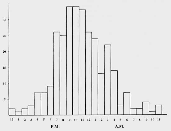
We examine now the actual data recorded for this study. Figure 9 displays the number of sightings per hour interval for all events. Figure 10 then presents the data for only those events that occurred in the United States and Canada,
Note how both distributions follow very closely the same pattern. This pattern has been described by Vallee as the Second Positive Law, or Law of the Times (2). Very few events are reported during the day; the reports increase sharply about 18:00 local time to a peak around 21 to 22:00, with a minor peak of sightings at 3:00 Vallee's reports were a mixture of those from vehicles and those not, with the majority from stationary observers. It is curious then, upon first consideration, that the EM event pattern adheres to this law, because while many people are out-of-doors in the early evening--hence the higher number of reports ? many more vehicles are on the road during the day than evening or night.
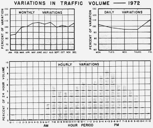
To investigate the matter further, data was gathered to determine the number of vehicles present on U.S. and Canadian highways by hour of the day. In the course of this search, it was discovered that such all-encompassing figures are not reported for the two countries as a whole.Instead, figures are given for selected localities, regions, or types of highway. Typical of this is Figure 11, depicting the variation of traffic in Sioux City, Iowa.
To make an adjustment for vehicles on the road, we must make the following approximations. Since the variance of EM events by month is peaked in October and November, we assume that the traffic flow per hour of the day does not vary much from one season to another. Mutatis mutandis, the same is true for variation of events by day of the week. Since the data spans over thirty years, we also assume that no significant change in driving habits, by hour of the day, has occurred in this period. These approximations appear to be valid, as any trends in the data are minor compared to the actual variation by hour in vehicles on the road.
| Heure du jour | % du volume journalier |
|---|---|
| 6:00 - 7:00 | 3.2% |
| 7:00 - 8:00 | 5.3% |
| 8:00 - 9:00 | 5.0% |
| 9:00 - 10:00 | 4.9% |
| 10:00 - 11:00 | 5.0% |
| 11:00 - 12:00 | 5.3% |
| 12:00 - 13:00 | 5.4% |
| 13:00 - 14:00 | 5.8% |
| 14:00 - 15:00 | 6.1% |
| 15:00 - 16:00 | 6.8% |
| 16:00 - 17:00 | 8.0% |
| 17:00 - 18:00 | 7.7% |
| 18:00 - 19:00 | 6.3% |
| 19:00 - 20:00 | 5.5% |
| 20:00 - 21:00 | 4.4% |
| 21:00 - 22:00 | 3.5% |
| 22:00 - 23:00 | 2.9% |
| 23:00 - 0:00 | 2.0% |
| 00:00 - 1:00 | 1.4% |
| 1:00 - 2:00 | 0.8% |
| 2:00 - 3:00 | 0.6% |
| 3:00 - 4:00 | 0.4% |
| 4:00 - 5:00 | 0.5% |
| 5:00 - 6:00 | 1.1% |
There are more vehicles on the highway and more miles driven in urban and suburban areas, as compared to rural areas (3). On the other hand, about two-thirds of the events occurred in rural or isolated areas. A study by Meyerhoff gives some global data for the United States, but no explanation is given as to how these statistics were derived (4). To calculate the hourly variation of traffic flow, additional results were used, including those from Sioux City, those from a rural state highway system, and an urban system (5, 6, 7). Simple linear averaging was used, with the U.S. figures from Meyerhoff given a weight of three versus single weights for other distributions. This was done to ensure that rural traffic would be adequately represented. In particular, giving equal weight to rural state highway statistics and those from an urban system actually gives greater emphasis to rural traffic, since there are far fewer vehicles in the rural area. The final figures are as shown in Table 12.
The percentages in Table 12 can only be approximate, given the nature of their derivation, but any observer familiar with traffic patterns would agree that they constitute a reasonable depiction of average traffic flow.
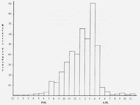
Using Table 12 and Figure 10, we then adjust the reported number of EM events, with reference to the fraction of a day in one hour, or 4.2%. If any hour's traffic flow exceeds that percentage, its absolute total is reduced, and vice versa. Figure 12 shows the results of such a calculation.
Comparing Figure 10 to Figure 12, we note a considerable change in the time distributions. While the highest frequencies in Figure 12 are still in the 18:00 ą 6:00 period, the peak has shifted to 3:00. A span of time between 23:00 et 5:00 now contains the bulk of the sightings.
What to make of Figure 12? First, if one believes that EM events are directed or planned, then it becomes merely the relative frequency or chance of any one driver experiencing an EM event by hour of the day. Note that during the period from 14:00 ą 15:00, the chance of experiencing an event is 131 times less than at 3:00 ! Still, the absolute chance of experiencing an EM event is very small; only about fifteen events are recorded per year, on the average (perhaps eight times that number may actually occur (8)).
If instead the three assumptions outlined previously are satisfied, Figure 12 can be considered to be the relative frequency of occurrence of EM events, in the United States and Canada, by hour of the day. The EM Phenomenon would thus occur 131 times more frequently at 3:00 than 14:00. If this interpretation is correct, this is an important piece of evidence bearing on the question of the nature of UFOs. For example, the hourly distribution of thunderstorms over the United States is highly skewed towards the late afternoon hours. This is a consequence of their method of formation, because the atmosphere must first be heated sufficiently to cause enough uplifting to form clouds of the correct type and size to cause thunderstorms. This does not usually happen until the late afternoon.
The fact that EM events peak around 3:00, and preferentially occur in those hours when few vehicles are on the highway, may therefore be a clue to the driving mechanism behind such events. Persinger has suggested that piezoelectric fields may be responsible for a majority of EM events (9); however, it does not seem plausible that such fields be preferentially formed in the hours between 23:00 and 5:00. Stress fractures and other similar tectonic events are caused by interactions between the earth, the moon, and the sun, plus complex internal geological mechanisms. There is no a priori reason to expect a non-random distribution of piezoelectric events by hour of the day.
It is important to observe that, if the above analysis of the meaning of Figure 12 cannot be accepted because one believes that EM events are always directed by some intelligence, then the results displayed in Figure 10 become the relative frequencies of EM events by hour of the day. Figure 12 can then be considered to be the relative chance of any driver experiencing an EM event. Conversely, if one attributes EM events to an intelligence which inadvertently causes them as a by-product of its activity, then Figure 12 again becomes the relative frequency of occurrence of EM events, and therefore also the relative chance of any driver experiencing an EM event. Figure 12, of course, can also be interpreted in this manner if EM events are not caused by some intelligence. Either Figure 10 or Figure 12 should be the "true" representation of hourly frequency. We simply don't have enough data to make a choice yet.